Overview
Contents
Overview#
The library#
All functionality in xlandsat is available from the base namespace of the
xlandsat package. This means that you can access all of them with a
single import:
# xlandsat is usually imported as xls
import xlandsat as xls
Download a sample scene#
As an example, lets download a tar archive of a Landsat 8 scene of the Brumadinho tailings dam disaster that happened in 2019 in Brazil. The archive is available on figshare at https://doi.org/10.6084/m9.figshare.21665630.v1 and includes scenes from before and after the disaster as both the full scene and a cropped version.
We’ll use pooch to download the scenes from before and after the
disaster to our computer.
To save space and bandwidth, we’ll use the cropped version here.
import pooch

path_before = pooch.retrieve(
      "doi:10.6084/m9.figshare.21665630.v1/cropped-before.tar.gz",
     known_hash="md5:d2a503c944bb7ef3b41294d44b77e98c",
)
path_after = pooch.retrieve(
      "doi:10.6084/m9.figshare.21665630.v1/cropped-after.tar.gz",
     known_hash="md5:4ae61a2d7a8b853c727c0c433680cece",
)
print(path_before)
print(path_after)
/home/runner/.cache/pooch/cc3e48c8ee8ca9c9ccb64e2a0e798286-cropped-before.tar.gz
/home/runner/.cache/pooch/7450bb0a799deea586280f7c3b539898-cropped-after.tar.gz
Tip
Running the code above will only download the data once since Pooch is
smart enough to check if the file already exists on your computer.
See pooch.retrieve for more information.
See also
If you want to use the full scene instead of the cropped version,
substitute the file name to full-after.tar.gz and
full-before.tar.gz. Don’t forget to also update the MD5 hashes
accordingly, which you can find on the figshare archive.
Load the scenes#
Now that we have paths to the tar archives of the scenes, we can use
xlandsat.load_scene to read the bands and metadata directly from the
archives (without unpacking):
before = xls.load_scene(path_before)
before
<xarray.Dataset>
Dimensions:   (easting: 400, northing: 300)
Coordinates:
  * easting   (easting) float64 5.835e+05 5.835e+05 ... 5.954e+05 5.955e+05
  * northing  (northing) float64 -2.232e+06 -2.232e+06 ... -2.223e+06 -2.223e+06
Data variables:
    blue      (northing, easting) float16 0.07288 0.07373 ... 0.06506 0.06653
    green     (northing, easting) float16 0.09851 0.099 ... 0.0835 0.08716
    red       (northing, easting) float16 0.1035 0.1041 ... 0.07959 0.08423
    nir       (northing, easting) float16 0.2803 0.2749 0.3203 ... 0.2118 0.2267
    swir1     (northing, easting) float16 0.2467 0.2474 0.2147 ... 0.172 0.1769
    swir2     (northing, easting) float16 0.1571 0.1571 0.1281 ... 0.1171 0.1206
Attributes: (12/62)
    Conventions:                     CF-1.8
    title:                           Landsat 8 scene from 2019-01-14 (path/ro...
    origin:                          Image courtesy of the U.S. Geological Su...
    digital_object_identifier:       https://doi.org/10.5066/P9OGBGM6
    landsat_product_id:              LC08_L2SP_218074_20190114_20200829_02_T1
    processing_level:                L2SP
    ...                              ...
    temperature_mult_band_st_b10:    0.00341802
    temperature_add_band_st_b10:     149.0
    reflectance_mult_band_8:         2e-05
    reflectance_mult_band_9:         2e-05
    reflectance_add_band_8:          -0.1
reflectance_add_band_9: -0.1And the after scene:
after = xls.load_scene(path_after)
after
<xarray.Dataset>
Dimensions:   (easting: 400, northing: 300)
Coordinates:
  * easting   (easting) float64 5.844e+05 5.844e+05 ... 5.963e+05 5.964e+05
  * northing  (northing) float64 -2.232e+06 -2.232e+06 ... -2.223e+06 -2.223e+06
Data variables:
    blue      (northing, easting) float16 0.0686 0.07043 ... 0.05823 0.0564
    green     (northing, easting) float16 0.1027 0.09839 ... 0.07593 0.07043
    red       (northing, easting) float16 0.09778 0.09778 ... 0.06799 0.06177
    nir       (northing, easting) float16 0.2988 0.2715 0.2881 ... 0.2637 0.251
    swir1     (northing, easting) float16 0.2311 0.2274 0.2316 ... 0.1608 0.142
    swir2     (northing, easting) float16 0.145 0.1442 0.144 ... 0.09961 0.08655
Attributes: (12/62)
    Conventions:                     CF-1.8
    title:                           Landsat 8 scene from 2019-01-30 (path/ro...
    origin:                          Image courtesy of the U.S. Geological Su...
    digital_object_identifier:       https://doi.org/10.5066/P9OGBGM6
    landsat_product_id:              LC08_L2SP_218074_20190130_20200829_02_T1
    processing_level:                L2SP
    ...                              ...
    temperature_mult_band_st_b10:    0.00341802
    temperature_add_band_st_b10:     149.0
    reflectance_mult_band_8:         2e-05
    reflectance_mult_band_9:         2e-05
    reflectance_add_band_8:          -0.1
reflectance_add_band_9: -0.1Did you notice?
If you look carefully at the coordinates for each scene, you may notice
that they don’t exactly coincide in area. That’s OK since xarray
knows how to take the pixel coordinates into account when doing
mathematical operations like calculating indices and differences between
scenes.
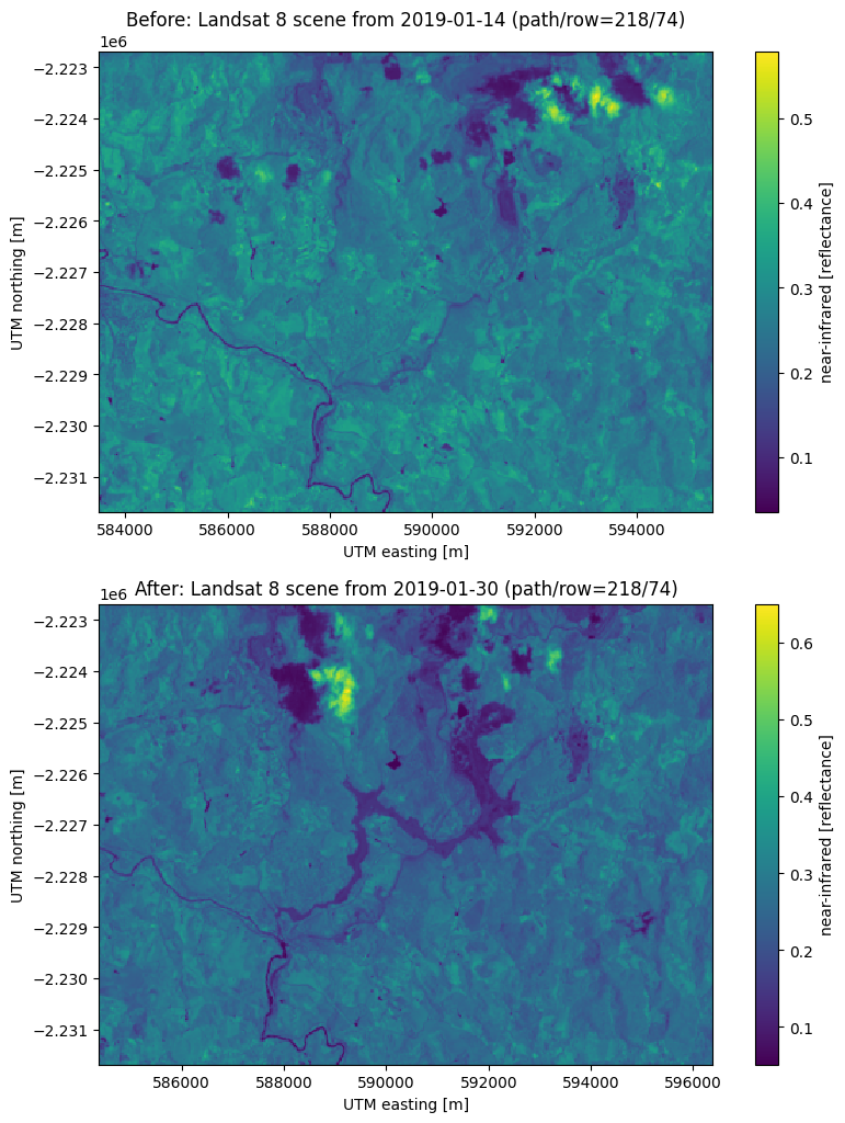
Plot some reflectance bands#
Now we can use the xarray.DataArray.plot method to make plots of
individual bands with matplotlib. A bonus is that xarray uses the
metadata that xlandsat.load_scene inserts into the scene to
automatically add labels and annotations to the plot.
import matplotlib.pyplot as plt

fig, (ax1, ax2) = plt.subplots(2, 1, figsize=(10, 12))

# Make the pseudocolor plots of the near infrared band
before.nir.plot(ax=ax1)
after.nir.plot(ax=ax2)

# Set the title using metadata from each scene
ax1.set_title(f"Before: {before.attrs['title']}")
ax2.set_title(f"After: {after.attrs['title']}")

# Set the aspect to equal so that pixels are squares, not rectangles
ax1.set_aspect("equal")
ax2.set_aspect("equal")

plt.show()
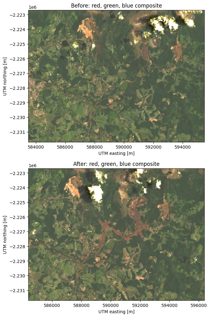
Make composites#
Plotting individual bands is good but we usually want to make some composite
images to visualize information from multiple bands at once.
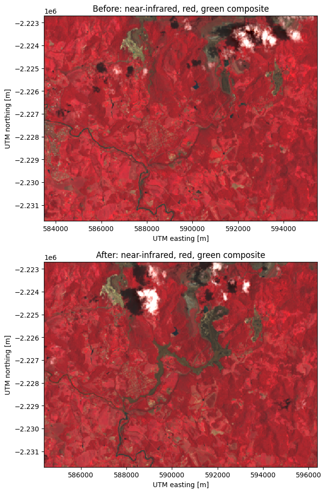
Let’s make both RGB (true color) and CIR (color infrared) composites for both
of our scenes using xlandsat.composite:
# Make the composite and add it as a variable to the scene
before = before.assign(rgb=xls.composite(before, rescale_to=[0, 0.2]))
cir_bands = ("nir", "red", "green")
before = before.assign(
    cir=xls.composite(before, bands=cir_bands, rescale_to=[0, 0.4]),
)
before
<xarray.Dataset>
Dimensions:   (easting: 400, northing: 300, channel: 4)
Coordinates:
  * easting   (easting) float64 5.835e+05 5.835e+05 ... 5.954e+05 5.955e+05
  * northing  (northing) float64 -2.232e+06 -2.232e+06 ... -2.223e+06 -2.223e+06
  * channel   (channel) <U5 'red' 'green' 'blue' 'alpha'
Data variables:
    blue      (northing, easting) float16 0.07288 0.07373 ... 0.06506 0.06653
    green     (northing, easting) float16 0.09851 0.099 ... 0.0835 0.08716
    red       (northing, easting) float16 0.1035 0.1041 ... 0.07959 0.08423
    nir       (northing, easting) float16 0.2803 0.2749 0.3203 ... 0.2118 0.2267
    swir1     (northing, easting) float16 0.2467 0.2474 0.2147 ... 0.172 0.1769
    swir2     (northing, easting) float16 0.1571 0.1571 0.1281 ... 0.1171 0.1206
    rgb       (northing, easting, channel) uint8 132 125 92 255 ... 111 84 255
    cir       (northing, easting, channel) uint8 178 66 62 255 ... 144 53 55 255
Attributes: (12/62)
    Conventions:                     CF-1.8
    title:                           Landsat 8 scene from 2019-01-14 (path/ro...
    origin:                          Image courtesy of the U.S. Geological Su...
    digital_object_identifier:       https://doi.org/10.5066/P9OGBGM6
    landsat_product_id:              LC08_L2SP_218074_20190114_20200829_02_T1
    processing_level:                L2SP
    ...                              ...
    temperature_mult_band_st_b10:    0.00341802
    temperature_add_band_st_b10:     149.0
    reflectance_mult_band_8:         2e-05
    reflectance_mult_band_9:         2e-05
    reflectance_add_band_8:          -0.1
reflectance_add_band_9: -0.1The composites have a similar layout as the bands but with an extra
"channel" dimension corresponding to red, green, blue, and
alpha/transparency. The values are scaled to the [0, 255] range and the
composite is an array of unsigned 8-bit integers.
Transparency
If any of the bands used for the composite have NaNs, those pixels will have their transparency set to the maximum value of 255. If there are no NaNs in any band, then the composite will only have 3 channels (red, green, blue).
Now do the same for the after scene:
after = after.assign(rgb=xls.composite(after, rescale_to=[0, 0.2]))
after = after.assign(
    cir=xls.composite(after, bands=cir_bands, rescale_to=[0, 0.4]),
)
after
<xarray.Dataset>
Dimensions:   (easting: 400, northing: 300, channel: 4)
Coordinates:
  * easting   (easting) float64 5.844e+05 5.844e+05 ... 5.963e+05 5.964e+05
  * northing  (northing) float64 -2.232e+06 -2.232e+06 ... -2.223e+06 -2.223e+06
  * channel   (channel) <U5 'red' 'green' 'blue' 'alpha'
Data variables:
    blue      (northing, easting) float16 0.0686 0.07043 ... 0.05823 0.0564
    green     (northing, easting) float16 0.1027 0.09839 ... 0.07593 0.07043
    red       (northing, easting) float16 0.09778 0.09778 ... 0.06799 0.06177
    nir       (northing, easting) float16 0.2988 0.2715 0.2881 ... 0.2637 0.251
    swir1     (northing, easting) float16 0.2311 0.2274 0.2316 ... 0.1608 0.142
    swir2     (northing, easting) float16 0.145 0.1442 0.144 ... 0.09961 0.08655
    rgb       (northing, easting, channel) uint8 124 131 87 255 ... 78 89 71 255
    cir       (northing, easting, channel) uint8 190 62 65 255 ... 160 39 44 255
Attributes: (12/62)
    Conventions:                     CF-1.8
    title:                           Landsat 8 scene from 2019-01-30 (path/ro...
    origin:                          Image courtesy of the U.S. Geological Su...
    digital_object_identifier:       https://doi.org/10.5066/P9OGBGM6
    landsat_product_id:              LC08_L2SP_218074_20190130_20200829_02_T1
    processing_level:                L2SP
    ...                              ...
    temperature_mult_band_st_b10:    0.00341802
    temperature_add_band_st_b10:     149.0
    reflectance_mult_band_8:         2e-05
    reflectance_mult_band_9:         2e-05
    reflectance_add_band_8:          -0.1
reflectance_add_band_9: -0.1Plot the composites#
Composites can be plotted using xarray.DataArray.plot.imshow (using
plot won’t work and will display histograms instead).
Let’s make the before and after figures again for each of the composites we
generated.
fig, (ax1, ax2) = plt.subplots(2, 1, figsize=(10, 12))

# Plot the composites
before.rgb.plot.imshow(ax=ax1)
after.rgb.plot.imshow(ax=ax2)

# The "long_name" of the composite is the band combination
ax1.set_title(f"Before: {before.rgb.attrs['long_name']}")
ax2.set_title(f"After: {after.rgb.attrs['long_name']}")

ax1.set_aspect("equal")
ax2.set_aspect("equal")

plt.show()
And now the CIR composites:
fig, (ax1, ax2) = plt.subplots(2, 1, figsize=(10, 12))

before.cir.plot.imshow(ax=ax1)
after.cir.plot.imshow(ax=ax2)

ax1.set_title(f"Before: {before.cir.attrs['long_name']}")
ax2.set_title(f"After: {after.cir.attrs['long_name']}")

ax1.set_aspect("equal")
ax2.set_aspect("equal")

plt.show()
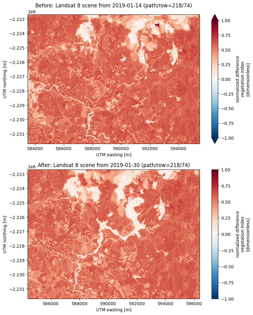
Calculating indices#
Producing indices from these scenes is straightforward thanks to
xarray’s excelled support for coordinate-aware operations.
As an example, let’s calculate the
NDVI:
before = before.assign(
    ndvi=(before.nir - before.red) / (before.nir + before.red),
)
after = after.assign(
    ndvi=(after.nir - after.red) / (after.nir + after.red),
)

# Set some metadata for xarray to find
before.ndvi.attrs["long_name"] = "normalized difference vegetation index"
before.ndvi.attrs["units"] = "dimensionless"
after.ndvi.attrs["long_name"] = "normalized difference vegetation index"
after.ndvi.attrs["units"] = "dimensionless"

after
<xarray.Dataset>
Dimensions:   (easting: 400, northing: 300, channel: 4)
Coordinates:
  * easting   (easting) float64 5.844e+05 5.844e+05 ... 5.963e+05 5.964e+05
  * northing  (northing) float64 -2.232e+06 -2.232e+06 ... -2.223e+06 -2.223e+06
  * channel   (channel) <U5 'red' 'green' 'blue' 'alpha'
Data variables:
    blue      (northing, easting) float16 0.0686 0.07043 ... 0.05823 0.0564
    green     (northing, easting) float16 0.1027 0.09839 ... 0.07593 0.07043
    red       (northing, easting) float16 0.09778 0.09778 ... 0.06799 0.06177
    nir       (northing, easting) float16 0.2988 0.2715 0.2881 ... 0.2637 0.251
    swir1     (northing, easting) float16 0.2311 0.2274 0.2316 ... 0.1608 0.142
    swir2     (northing, easting) float16 0.145 0.1442 0.144 ... 0.09961 0.08655
    rgb       (northing, easting, channel) uint8 124 131 87 255 ... 78 89 71 255
    cir       (northing, easting, channel) uint8 190 62 65 255 ... 160 39 44 255
    ndvi      (northing, easting) float16 0.5073 0.4705 0.4907 ... 0.5903 0.605
Attributes: (12/62)
    Conventions:                     CF-1.8
    title:                           Landsat 8 scene from 2019-01-30 (path/ro...
    origin:                          Image courtesy of the U.S. Geological Su...
    digital_object_identifier:       https://doi.org/10.5066/P9OGBGM6
    landsat_product_id:              LC08_L2SP_218074_20190130_20200829_02_T1
    processing_level:                L2SP
    ...                              ...
    temperature_mult_band_st_b10:    0.00341802
    temperature_add_band_st_b10:     149.0
    reflectance_mult_band_8:         2e-05
    reflectance_mult_band_9:         2e-05
    reflectance_add_band_8:          -0.1
reflectance_add_band_9: -0.1And now we can make pseudocolor plots of the NDVI:
fig, (ax1, ax2) = plt.subplots(2, 1, figsize=(10, 12))

# Limit the scale to [-1, +1] so the plots are easier to compare
before.ndvi.plot(ax=ax1, vmin=-1, vmax=1, cmap="RdBu_r")
after.ndvi.plot(ax=ax2, vmin=-1, vmax=1, cmap="RdBu_r")

ax1.set_title(f"Before: {before.attrs['title']}")
ax2.set_title(f"After: {after.attrs['title']}")

ax1.set_aspect("equal")
ax2.set_aspect("equal")

plt.show()
Finally, we can calculate the change in NDVI from one scene to the other by taking the difference:
ndvi_change = before.ndvi - after.ndvi
ndvi_change.name = "ndvi_change"
ndvi_change.attrs["long_name"] = (
    f"NDVI change between {before.attrs['date_acquired']} and "
    f"{after.attrs['date_acquired']}"
)
ndvi_change
<xarray.DataArray 'ndvi_change' (northing: 300, easting: 370)>
array([[ 0.05908 ,  0.06323 ,  0.0542  , ...,  0.004395, -0.009766,
         0.07324 ],
       [ 0.0498  ,  0.07764 ,  0.07495 , ...,  0.0957  ,  0.012695,
         0.003906],
       [-0.010254,  0.11743 ,  0.0747  , ...,  0.03125 ,  0.01807 ,
         0.04004 ],
       ...,
       [-0.000977,  0.01123 ,  0.000977, ...,  0.00928 ,  0.01367 ,
         0.00708 ],
       [ 0.00879 ,  0.02344 ,  0.01318 , ...,  0.006836,  0.00586 ,
         0.001221],
       [-0.01221 ,  0.02637 ,  0.006836, ...,  0.01343 ,  0.01221 ,
         0.0105  ]], dtype=float16)
Coordinates:
  * easting   (easting) float64 5.844e+05 5.844e+05 ... 5.954e+05 5.955e+05
  * northing  (northing) float64 -2.232e+06 -2.232e+06 ... -2.223e+06 -2.223e+06
Attributes:
long_name: NDVI change between 2019-01-14 and 2019-01-30Did you notice?
The keen-eyed among you may have noticed that the number of points along
the "easting" dimension has decreased. This is because xarray
only makes the calculations for pixels where the two scenes coincide. In
this case, there was an East-West shift between scenes but our calculations
take that into account.
Now lets plot it:
fig, ax = plt.subplots(1, 1, figsize=(10, 6))
ndvi_change.plot(ax=ax, vmin=-1, vmax=1, cmap="RdBu_r")
ax.set_aspect("equal")
plt.show()
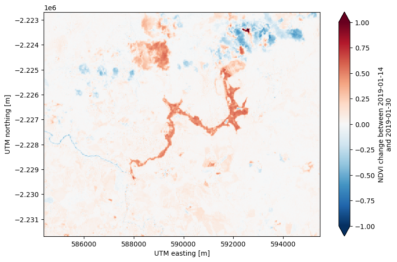
There’s some noise in the cloudy areas of both scenes in the northeast but otherwise this plots highlights the area affected by flooding from the dam collapse in bright red at the center.
What now?#
By getting the data into an xarray.Dataset, xlandsat opens the door
for a huge range of operations. You now have access to everything that
xarray can do: interpolation, reduction, slicing, grouping, saving to
cloud-optimized formats, and much more. So go off and do something cool!