Indices#

Indices calculated from multispectral satellite imagery are powerful ways to quantitatively analyze these data. They take advantage of different spectral properties of materials to differentiate between them. Many of these indices can be calculated with simple arithmetic operations. So now that our data are in xarray.Dataset’s it’s fairly easy to calculate them.

NDVI#

As an example, let’s load two example scenes from the Brumadinho tailings dam disaster:

import xlandsat as xls
import matplotlib.pyplot as plt

path_before = xls.datasets.fetch_brumadinho_before()
path_after = xls.datasets.fetch_brumadinho_after()

before = xls.load_scene(path_before)
after = xls.load_scene(path_after)

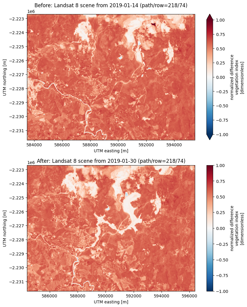
We can calculate the NDVI for these scenes to see if we can isolate the effect of the flood following the dam collapse:

And now we can make pseudo-color plots of the NDVI:

fig, (ax1, ax2) = plt.subplots(2, 1, figsize=(10, 12))

# Limit the scale to [-1, +1] so the plots are easier to compare
before.ndvi.plot(ax=ax1, vmin=-1, vmax=1, cmap="RdBu_r")
after.ndvi.plot(ax=ax2, vmin=-1, vmax=1, cmap="RdBu_r")

ax1.set_title(f"Before: {before.attrs['title']}")
ax2.set_title(f"After: {after.attrs['title']}")

ax1.set_aspect("equal")
ax2.set_aspect("equal")

plt.show()

Finally, we can calculate the change in NDVI from one scene to the other by taking the difference:

Did you notice?

The keen-eyed among you may have noticed that the number of points along the "easting" dimension has decreased. This is because xarray only makes the calculations for pixels where the two scenes coincide. In this case, there was an East-West shift between scenes but our calculations take that into account.

Now lets plot it:

fig, ax = plt.subplots(1, 1, figsize=(10, 6))
ndvi_change.plot(ax=ax, vmin=-1, vmax=1, cmap="PuOr")
ax.set_aspect("equal")
plt.show()

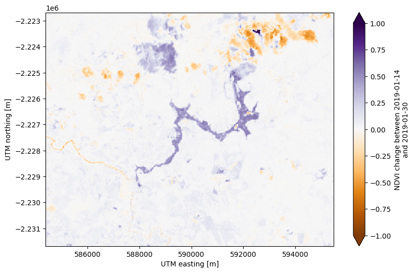
There’s some noise in the cloudy areas of both scenes in the northeast but otherwise this plots highlights the area affected by flooding from the dam collapse in bright red at the center.

xlandsat v0.3.0

Indices

Contents

Indices#

NDVI#