Pansharpening#

Landsat includes a panchromatic band which has greater spatial resolution (15 m versus the standard 30 m of visible bands). It can be used to artificially increase the resolution of the visible bands (red, green, and blue) in a process called pansharpening.

To illustrate this concept, let’s download a scene from just North of the city of Liverpool, UK:

import xlandsat as xls
import matplotlib.pyplot as plt

path = xls.datasets.fetch_liverpool()
path_pan = xls.datasets.fetch_liverpool_panchromatic()

Load the scene with xlandsat.load_scene:

And load the panchromatic band with xlandsat.load_panchromatic:

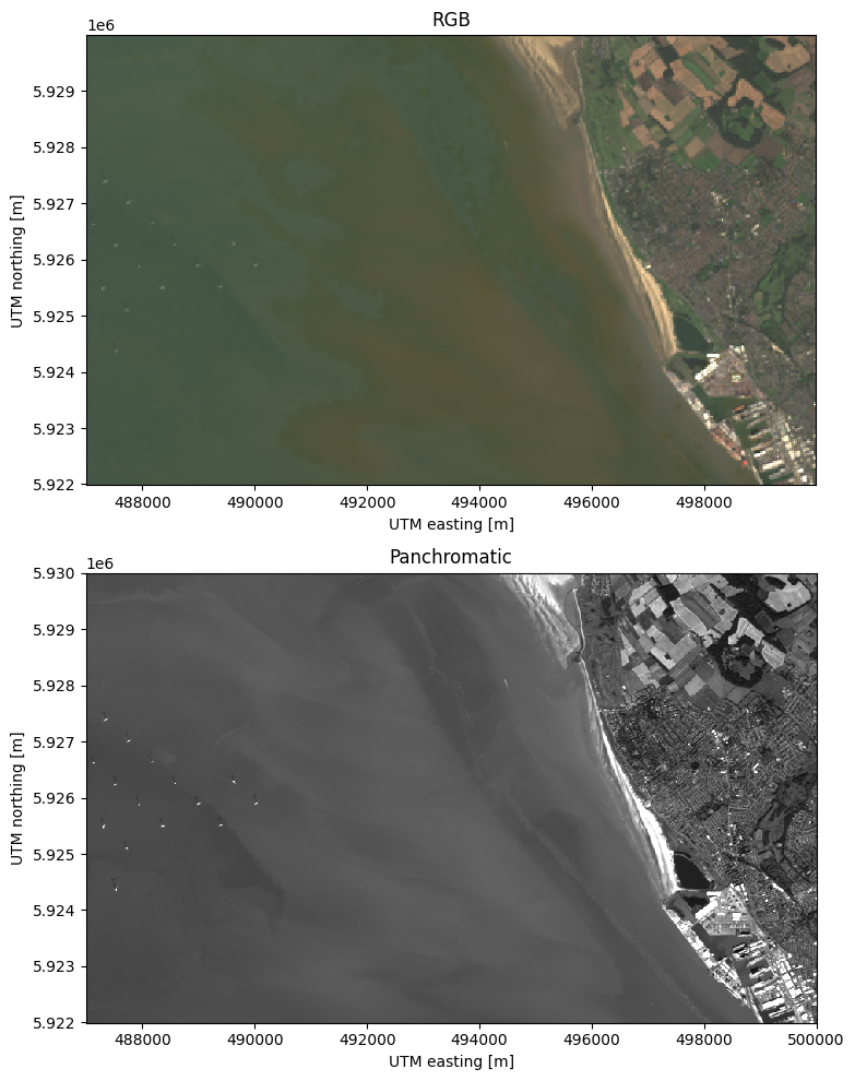
Now we can plot an RGB composite and the panchromatic band for comparison:

rgb = xls.composite(scene, rescale_to=(0, 0.25))

plt.figure(figsize=(16, 10))
ax = plt.subplot(2, 1, 1)
rgb.plot.imshow(ax=ax)
ax.set_aspect("equal")
ax.set_title("RGB")
ax = plt.subplot(2, 1, 2)
panchromatic.plot.pcolormesh(
    ax=ax, cmap="gray", vmin=0.02, vmax=0.1, add_colorbar=False,
)
ax.set_aspect("equal")
ax.set_title("Panchromatic")
plt.tight_layout()

The pansharpening is implemented in xlandsat.pansharpen:

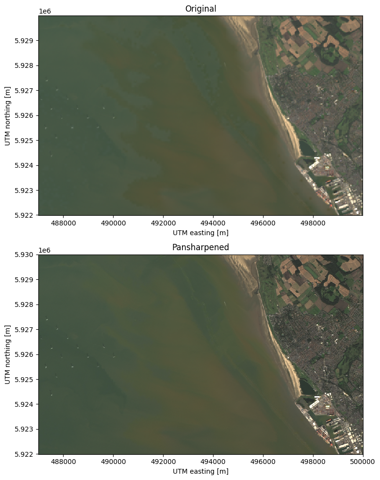
Finally, let’s compare the sharpened and original RGB composites:

rgb_sharp = xls.composite(scene_sharp, rescale_to=(0, 0.15))

plt.figure(figsize=(16, 10))
ax = plt.subplot(2, 1, 1)
rgb.plot.imshow(ax=ax)
ax.set_aspect("equal")
ax.set_title("Original")
ax = plt.subplot(2, 1, 2)
rgb_sharp.plot.imshow(ax=ax)
ax.set_aspect("equal")
ax.set_title("Pansharpened")
plt.tight_layout()